GLOBAL GEOCHEMICAL ATLASSKILL · global-geochemical-atlas 🏆 Champion
🏆 Champion · SynMatAI AI4S Future ScienceSkills Hackathon CHAMPION · TEAM TOKEN AGENTS ↗
AI4S Future ScienceSkills Hackathon · 🏆 Champion

Global Geochemical AtlasA reusable research skill for AI agents

A question that sounds simple · from a geochemist

“Map global arsenic in soil, organize it into an interactive database, and tell me where it is anomalous.”

It sounds like a retrieval task. Inside a real research team it immediately becomes four harder questions:

🧪 Geochemist

Dozens of surveys, three units, five digestion methods — can these numbers share one map at all?

→ Unified metrics
🏛️ Regulator

Arsenic in the southwest is several times the national median — pollution, or simply the geological background?

→ Temporal dynamics
🗂️ Data steward

This record is from 1978 — are its detection limit, coordinate system and license still traceable today?

→ Quality control
⚖️ Reviewer

For every number the AI produces, which page and which row does it come from? Would you dare cite it?

→ Provenance

How can one sentence make an agent deliver a trustworthy, traceable, interactive atlas of global element distribution that also evolves through time? The Global Geochemical Atlas Skill turns the different demands of different researchers into a single agent-native workflow: trustworthy, interactive, traceable, unified, and dynamic in time.

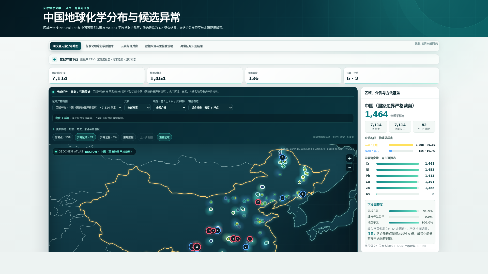
The world atlas is a self-contained 96 MB file; the first load takes a moment, and it keeps working offline once saved. Also available: Europe ↗ · China ↗ · temporal evolution map ↗.

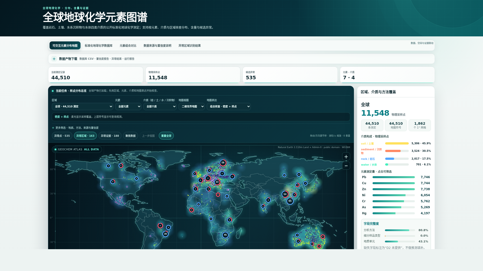
world-atlas.html · self-contained single file · click to open● LIVE
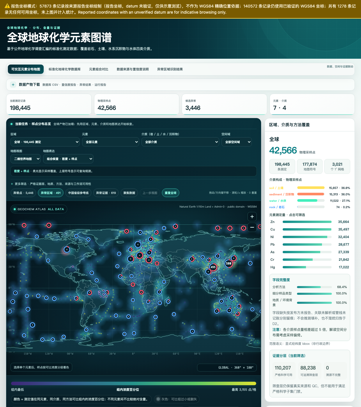
World atlas interface: global distribution of 198,445 measurements, anomaly candidate rings and the media coverage sidebar
Real run output — interface captureMAP / DATABASE / EVIDENCE
Acquire36 SOURCES Standardizemg/kg · WGS84 QC & repairITERATION LOOP Screen anomaliesROBUST-Z · FDR Attribute in timeGEOGENIC / INPUT Draft papers5 SCIENTIFIC QUESTIONS

Multi-source acquisition + standardization gates + QC repair loop = a trustworthy global element atlas, and papers

Team Affiliations
Shanghai Jiao Tong University
Beijing Zhongguancun Academy
Beihang University
Zhejiang University
Latest Production Run 2026-08-19 · global online production run · fully autonomous
199,730measurements admitted
no double counting
45,753distinct physical samples
rock / soil / sediment / water
35public sources admitted
31 further candidates audited and rejected
100%record-level provenance
all 199,730 records trace to their origin
3,721anomaly screening candidates
robust-z gate · 19 candidate regions
393records failed the standardization gate
kept honestly in place, never silently dropped

Honest reporting: the figures above come from the structured report embedded in the 2026-08-19 production outputs and can be checked item by item; coverage of Russia, South America and other regions is still thin and is kept as an explicit gap — this breadth is not a global statistical distribution. RUN A in the “Real-run evidence” section below is a separate 2026-08-15 run with its own accounting and is never mixed with this one; the online world atlas file carries its own tally of 36 sources / 199,723 plottable records — the difference from the run report reflects what each file counts, and both can be verified inside their respective files.

The Challenge

What the hackathon asked for

Climate & Earth Science track, task “Global Geochemical Element Distribution Atlas”: start from public data, complete the full chain of acquisition, processing, mapping and anomaly identification, and distil the workflow into a reusable Skill document.

01Automatic acquisitionACQUIRE

Collect element concentrations, sampling coordinates, geological background and analytical-method information for four media — rock, soil, sediment and water — from public literature and open data platforms.

02Scientific processingSTANDARDIZE

Perform unit unification, spatial matching, quality control and provenance tracing. This project adds one rule of its own: original measured values are never overwritten — converted values are stored in separate columns.

03Research outputsVISUALIZE

Render global or regional distribution maps, heatmaps and element-combination comparisons by element / region / geological unit / sample type, and identify anomalous enrichment and depletion areas.

04Skill outputsOUTPUTS

Produce an interactive element distribution map, a standardized geochemical database, source and confidence documentation, anomaly identification results and a reusable Skill document; the hackathon’s final deliverable is a single complete, reusable Skill document.

This page keeps the two layers apart: one run produces four kinds of research results; the reusable Skill document defines and reproduces the workflow — and is the final submission → see the run outputs

Skill Outputs · Runtime + Reusable Asset

Run outputs and the reusable Skill document

A single run produces the interactive map, the standardized database, the source & confidence documentation and the anomaly identification results; the reusable Skill document defines the workflow, the scientific gates and the output contract — it drives the run and is the final submission. All four results share one data foundation, one evidence chain and one set of scientific boundaries, and every one of them can be opened and verified here.

OUTPUT 1Interactive element distribution map

Interactive element distribution map

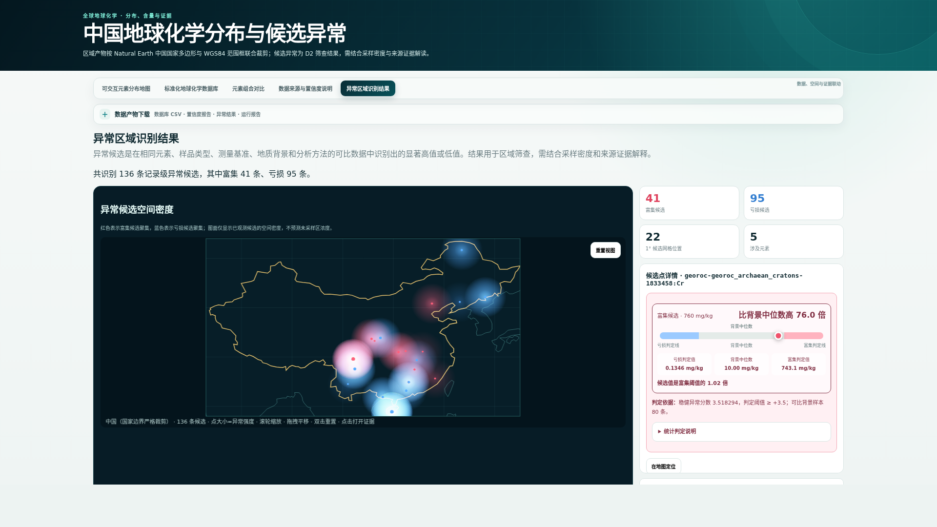
Enter any view by element, region, geological unit or sample type; sources with reliable time fields can be shown as a temporal evolution view; every point links straight to its original evidence.

OUTPUT 2Standardized geochemical database

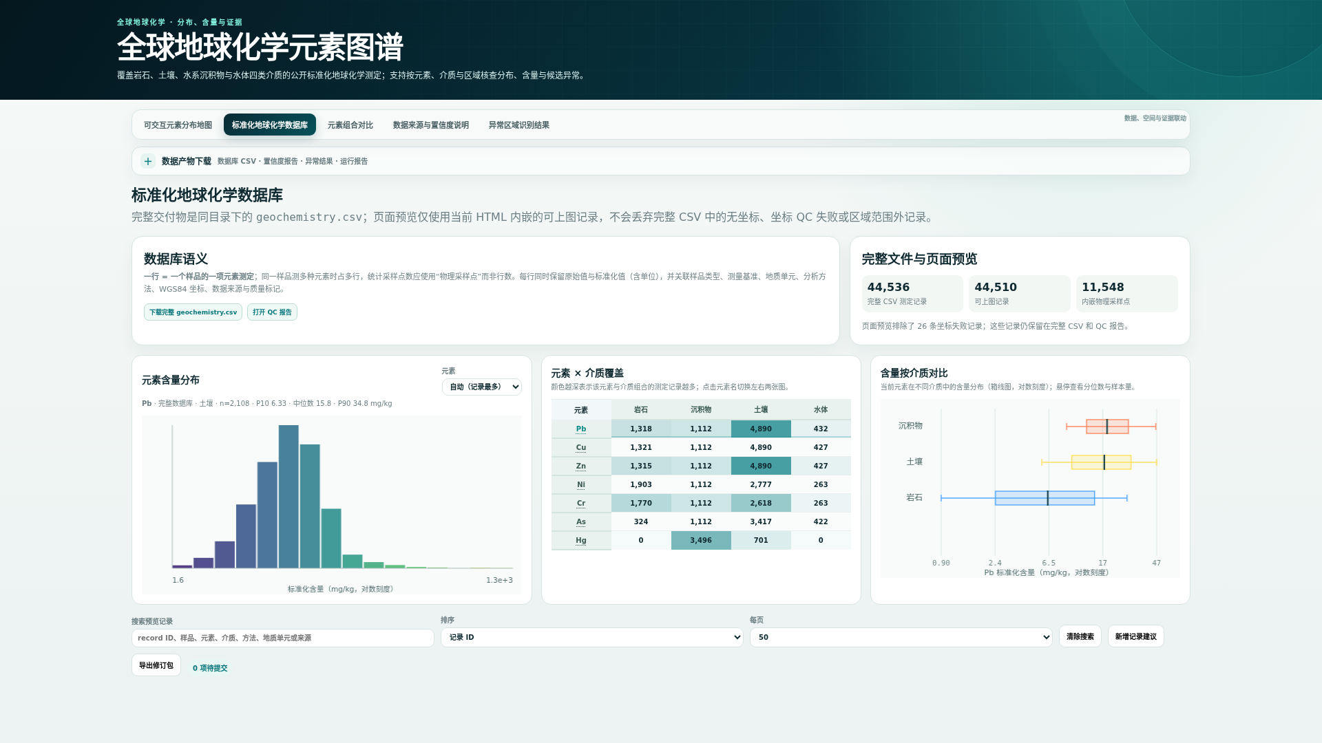
Standardized geochemical database

Long-table structure aligned with ODM2 semantics: units unified to mg/kg, coordinates to WGS84, original values never overwritten — the downloadable CSV is the standardized database itself.

OUTPUT 3Source and confidence documentation

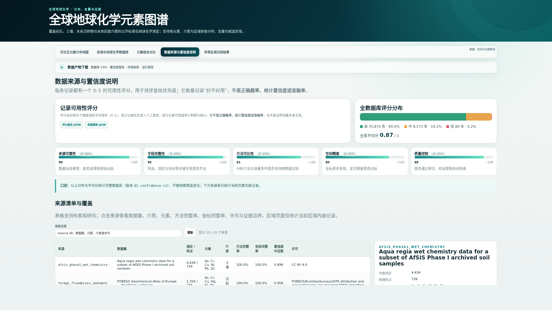
Source & confidence documentation

Every record carries a 0–1 usability score (five weighted components); every source carries its license, coverage and access notes; evidence drills down DOI → table / row → SHA-256.

OUTPUT 4Anomaly identification results

Anomaly identification results

Enrichment and depletion are reported separately; every candidate carries its statistical criteria and a review entry point. A candidate is not a mineralization verdict — the review chain leads back to the original records.

EXTRA3D globe view

3D globe and anomaly perspective

The same data on a three-dimensional globe: global sampling coverage and the pattern of anomalies at a glance.

SKILL DOCUMENT
$ opencode run "global Cr·Cu·Ni·Pb·Zn atlas with anomaly screening"
[agent] reading SKILL.md → nine-stage state machine
[agent] validate_outputs PASS · 18/18 artifacts

Reusable Skill document

Four layers: the SKILL.md state machine + a scientific knowledge base + deterministic executors + reproducible tests. Any compatible agent mounts it and runs; all numerical work is done by scripts — the model never touches the numbers.

How It Works · Six Design Commitments

How it works: six design commitments

Six mechanisms were presented at the final. This section explains, one by one, how each is actually done in code: the foot of every card names the script that implements it and the run evidence on this page you can open to check it.

Models propose, code decidesModels only nominate candidates, raise objections and write prose. Arithmetic, gate decisions and hash checks are all done by deterministic scripts; the model never touches the result. When something goes wrong, it can be traced back to a specific line of code rather than to a conversation.
01A complete iteration loop

The main line is nine steps and three gates: can a source come in, do units and coordinates pass QC, and does every item pass acceptance. Whatever fails goes into the repair loop; the bar is never lowered to let it through.

The repair loop has five steps, shown below. Every repair is a new run, and earlier evidence files are never rewritten. Problems that genuinely cannot be fixed are flagged needs_human_review and handed to a person instead of being patched with a made-up number. The whole chain can be driven by autopilot.py in one command, which ends in one of four machine-readable states: DONE / CONTINUE_REQUIRED / NEEDS_HUMAN_REVIEW / FAILED.

list the problemslog to backlogfix by registered methodre-run & re-acceptwrite to cross-run memory
02Three-layer adversarial mechanism

Adversaries sit at two points: where data comes in, and where results go out. The third layer is a graded verdict that decides whether a problem sends the work back, narrows its scope, or lets it through.

At the entrance there is a three-party duel: one model acts as the scout and nominates new data sources; a second model acts as the skeptic and may only raise problems, never score; the scoring is done by code against a fixed scoreboard — 7 points or more proceeds to onboarding, 4 to 6 is sent back for revision, below 4 is out. At the exit there is an output audit: the audit script first copies the outputs into a shadow copy, plants 10 known defect types in it (altered values, flipped units, fabricated sources, corrupted hashes and so on) and sits the exam itself. Only if it catches all 10 does its verdict on the real outputs count; miss one and the verdict is void. The verdict has three grades, pass / pass_scope_narrowed / fail: a warning does not kill the draft, but the affected numbers may only be quoted together with their scope.

03Each evaluation round stays independent

A round must be reviewed without being influenced by the previous round’s conclusions. This is written into a machine-readable reviewer contract, not left to convention.

The contract requires the skeptic to come from a different model family than the executor, to work in a brand-new thread, to see none of the executor’s explanations, and to read only the output files themselves; if a path or SHA-256 in the briefing does not match, it must refuse to review. As for cross-run memory (memory.json), it records only how often each source has succeeded or failed before, and its sole effect is the order in which round 1 tries sources: it cannot add a source and takes part in no decision. Evidence gathered in the current run always outranks memory from earlier ones.

04SHA-256 fingerprints, one per result

Hashes are taken in four places: the task request itself, every downloaded source file, the 18 output files, and every number in the final answer.

The request is hashed before work starts, so a goal that drifts midway shows up; source files must pass a registered hash check before ingestion; run_summary.json records the hash of each of the 18 outputs. The last layer is the claim ledger: claim_ledger.py lists every number in the outputs that could be quoted in an answer and binds each one to a file, a JSON pointer and a hash, recomputing all of it on every call so the executor cannot edit it. Once the answer is drafted, --check-answer compares it against the ledger; a number that does not match is treated as a phantom and may not be published. Inside the atlas, any point can likewise be followed down to its DOI, the row of the original table and the hash.

05Temporal evolution lives inside the atlas

Temporal evolution is not a separate deliverable. It is a view inside the atlas: switch to it and it is there, running on the same standardized database.

For sources with reliable sampling dates, the atlas can play year by year from 1986 to 2024, which helps tell whether a high value has always been the geological background or appeared later as an external input. Because it uses the same data, the evidence chain and the scientific boundaries of the main view hold in the temporal view too; there is no second set of accounting to maintain.

06Auto-research genuinely wired in

Once the atlas is built and has passed validation, you can choose to take one more step into research mode. The step is optional, and it is really connected — not a sentence in the documentation.

build_research_products.py collects no new data and changes no core output. It only reorganizes the existing evidence into three things a researcher can use directly: which records may be compared with one another (analysis cohorts), the lithology, depositional setting and other context of every sample (research context), and where to sample next (sampling priorities), with a receipt stating the input hashes and parameters. Research mode then continues on top of these three with statistical tests, writing and typesetting. The five papers further down this page were produced exactly this way.

Quick Start · Use It with Your Agent

Quick start: run it inside your own agent

The default prompt is the complete hackathon task; change three words and it is your task. Running it needs no network, API key, GPU or third-party package — Python 3.10+ is enough.

1Mount the skill

The skill folder follows the Agent Skills public subset (SKILL.md + references/ + scripts/ + assets/, pure standard library); copy it into a compatible runtime’s skills directory and you are done.

git clone https://github.com/asimfish/global-geochemical-atlas-skill
# Claude Code
cp -r global-geochemical-atlas-skill/skills/global-geochemical-atlas ~/.claude/skills/
# Codex CLI
cp -r global-geochemical-atlas-skill/skills/global-geochemical-atlas ~/.codex/skills/
# OpenCode and other compatible runtimes: copy / mount into their skills folder

Once mounted, the agent reads the nine-stage state machine in SKILL.md whenever a matching request arrives; the 5 should-activate and 4 adjacent should-not-activate cases in activation.json ↗ show where that boundary lies.

Python 3.10+no networkno API keyno GPUno third-party packages
2Send the default prompt to your agent and change only three slots

This prompt covers every step of the hackathon task description word for word. Replace the highlighted medium / element / region with yours — say, “Western Europe” with “China” — and it is your task.

Using only public literature and open data platforms, build a soil arsenic (As) atlas for Western Europe: automatically collect element concentrations, sampling coordinates, geological background, and analytical-method information; unify units, spatially match records, run quality control, and trace every record to its source; render the distribution map, heatmap, and element-combination comparison, filterable by element, region, geological unit, and sample type; identify candidate enrichment and depletion areas; and deliver the interactive atlas, the standardized geochemical database, the source & confidence documentation, and the anomaly identification results.

SLOTWHAT TO PUT THEREEXAMPLES
regionglobal, a named region, or a WGS84 bounding boxWestern Europe · China · lat 30–45, lon –10–30
mediumone or more of the four supported mediasoil · sediment · water · rock
elementelement symbol or analyte namearsenic (As) · Cu · Pb · Hg

Shorter requests activate the skill just as well, e.g. “Using only public data, build a soil arsenic atlas for Western Europe: standardize the units, flag candidate enrichment areas, and attach per-record sources, licenses, and confidence scores.” The full tutorial — three ways to run (your own data / online acquisition / the offline four-media sample), how to write request.json, and the FAQ — is in the GitHub README ↗.

3Or skip the agent: reproduce locally in 90 seconds

From the repository root, run the production-threshold demo on 996 hash-pinned real USGS soil measurements, then validate the 18-file output contract. The two commands should return partial_success and valid respectively.

python skills/global-geochemical-atlas/scripts/run_atlas_request.py \
  --request skills/global-geochemical-atlas/fixtures/production-usgs/request.json \
  --demo production-usgs --analysis-profile production \
  --generated-at 2026-08-07T00:00:00Z --output-dir /tmp/geochemical-production-demo
python skills/global-geochemical-atlas/scripts/validate_outputs.py \
  --output-dir /tmp/geochemical-production-demo

To let the conductor drive everything in one command (freeze the prompt → route → repair loop → validate → adversarial audit):

python skills/global-geochemical-atlas/scripts/autopilot.py \
  --prompt-file TASK_PROMPT.txt --output-dir /tmp/atlas-run
4After the atlas: optionally continue into the research layer

On top of any run that has completed and passed validation, one command turns the existing evidence into three researcher products (no new data, no changes to core outputs) with a receipt stating the input hashes. The five papers below started from this step.

  • analysis_cohorts.csv analysis cohorts: which records may be compared with one another, which may not, and why
  • research_context.csv research context: per-sample lithology, geological unit, depositional setting, depth, grain size and sampling date
  • sampling_priority.geojson sampling priorities: data gaps ranked into the next acquisition queue
  • research_products_receipt.json receipt: input hashes, parameters, and an explicit list of what may not be claimed
python skills/global-geochemical-atlas/scripts/build_research_products.py \
  --output-dir /tmp/atlas-run --research-dir /tmp/atlas-run/research \
  --minimum-confidence medium
Reproducibility · Real-Run Evidence

Validated in real runs: online acquisition, deterministic regression, adversarial audit

Three kinds of validation cover different risk surfaces: an online production run tests autonomous acquisition, failure handling and gap reporting under real network conditions; a deterministic regression in a fresh clone tests whether the core outputs reproduce byte for byte across environments; and an adversarial audit plants 10 artificial defect types in a shadow copy of the outputs to calibrate the auditor’s detection power. The three results use separate accounting and are never mixed.

RUN A · GLOBAL ONLINE PRODUCTION RUN · 2026-08-15

33 minutes online, worldwide: acquisition and consolidation completed autonomously, results and gaps reported honestly

  • 63 source candidates audited → 31 formally routed → 29 actually ingested
  • 9 acquisition rounds, 72,346 → 191,715 measurements; stopped on its own once increments reached zero
  • Two GEOROC endpoints kept returning HTTP 500 — failed closed round after round and recorded as such
  • 238-item repair queue retained; terminal state needs_human_review
RUN B · DETERMINISTIC REGRESSION · main@ed8249e

Regression completed in 0.714 s in a fresh clone: core outputs identical byte for byte

  • 996 measurements · 996/996 matched to geology · 6 candidates
  • All 15 core artifacts passed independent validation (that version’s contract had 15 files; it now has 18), 0 errors / 0 warnings
  • Hash-bound real-source fixture; re-runs across environments reproduce byte for byte
  • Proves engineering executability and the scientific gates — not a regional distribution
RUN C · ADVERSARIAL AUDIT DRILL · 2026-08-20

A red team planted 10 defect types, all caught: the audit layer is calibrated before it judges

  • Full chain with no human intervention: request freeze → pipeline run → output validation → adversarial audit → claim ledger (a fixed 1,422-record fixture built to exercise the audit layer)
  • 10 defect types planted in a shadow copy (value tampering, unit flips, fabricated sources, corrupted hashes, …); the auditor caught 10/10
  • 10 independent re-checks of the real outputs all passed (hash chain, unit recomputation, anomaly recomputation, …), 0 errors / 0 warnings
  • The claim ledger ruled the planted hallucinated number “25000” answer_unbound — numbers without an evidence binding may not appear in the answer; the executor can drive repairs, but cannot acquit itself

Scientific boundary: every anomaly is a screening candidate — not a conclusion about pollution, mineralization or genesis; censored values keep their qualifier and are never imputed as 0; the manifest, record-level locators and SHA-256 hashes are the final authority for every conclusion.

Beyond Atlas · Data → Papers

From atlas to discovery to papers: one continuous research workflow

A distribution map answers “what is where, and how much”; research has to answer “why, and what it means”. This skill joins the two into one workflow: once the atlas is built, discovery mode starts from the same frozen data snapshot, identifies testable signals in the data, turns them into candidate scientific questions, and then carries them through statistical testing, writing and typesetting — from element atlas, to data insight, to a complete piece of research, without ever switching tools. The workflow has run end to end five times and delivered five genuine findings: a century of atmospheric mercury and lead deposition left a detectable vertical fingerprint in European soils; that enrichment is absent in Australia — it is a regional signature of Northern Hemisphere industry, not a global norm; the same soil sample measured by a different method can differ threefold, and the offset can be modelled and converted; two mutually unaware continental surveys agree to within 2% on arsenic at the same locations, giving the global arsenic risk map its first independent ground validation; and a statistical layer with no oceanographic prior recovers textbook ocean profiles with zero tuning. Every number can be recomputed from the frozen snapshot with fixed-seed scripts; each paper below shows one methods figure and one main result.

P1
Legacy mercury and lead enrichment in European soil profiles: a method-stratified test QUESTIONHow strong a vertical signal has a century of atmospheric Hg/Pb deposition left in European soils? Does mixing analytical methods create artefacts?
10 pages · 4 figures, 1 table STOTEN / Applied Geochemistry Read the PDF ↗

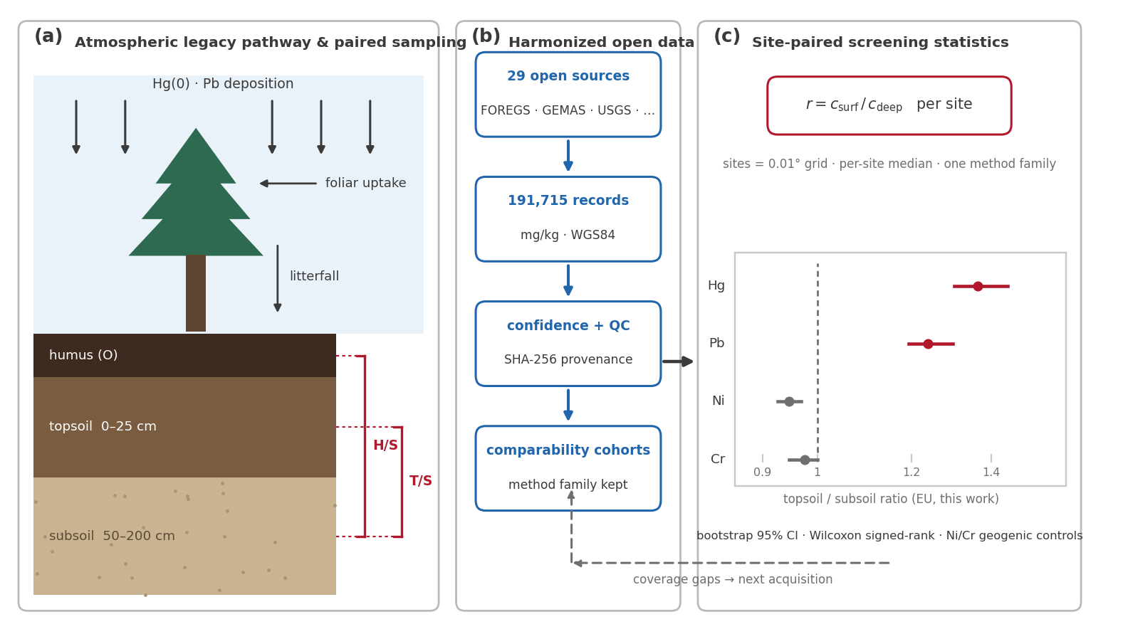
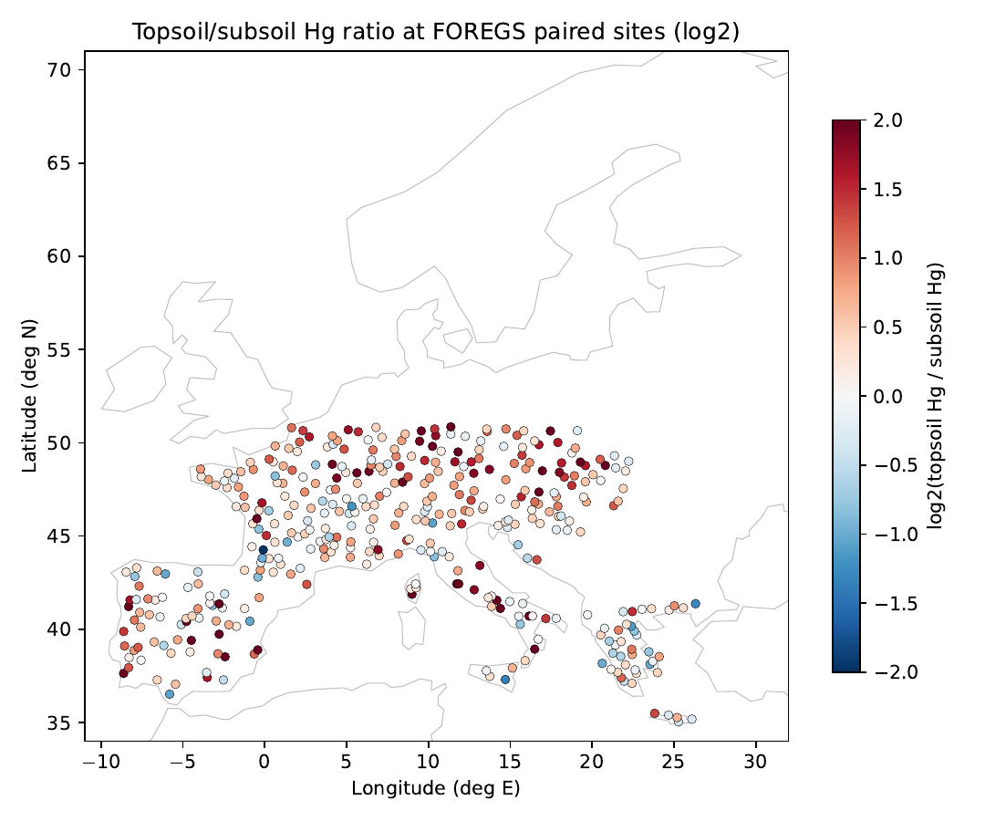
Finding: topsoil/subsoil concentration ratios are 1.36 for Hg and 1.24 for Pb — significant surface enrichment — while the geogenic reference elements Ni and Cr sit at ≈1, supporting an atmospheric-deposition origin rather than parent-rock differences. Hg in the humus layer reaches 5.3×, consistent with vegetation-mediated deposition and surface retention. Because the same element can differ threefold across methods, all statistics are stratified by method family first; the independent LUCAS survey gives a European topsoil Hg median consistent with this study (43.9 vs 38.3 µg/kg).

P1 methods figure
METHODSAtmospheric-deposition hypothesis → paired-site design → method-stratified statistics (three panels)
P1 results figure
RESULTMap of topsoil/subsoil Hg ratios at paired FOREGS sites: widespread red across Europe = surface enrichment
P2
Surface legacy enrichment is not a global norm: the Australian test QUESTIONIs the surface Pb enrichment of European soils a worldwide phenomenon or a regional signal of Northern Hemisphere industry? What does the Southern Hemisphere show under identical accounting?
9 pages · 5 figures, 1 table Environmental Pollution Read the PDF ↗

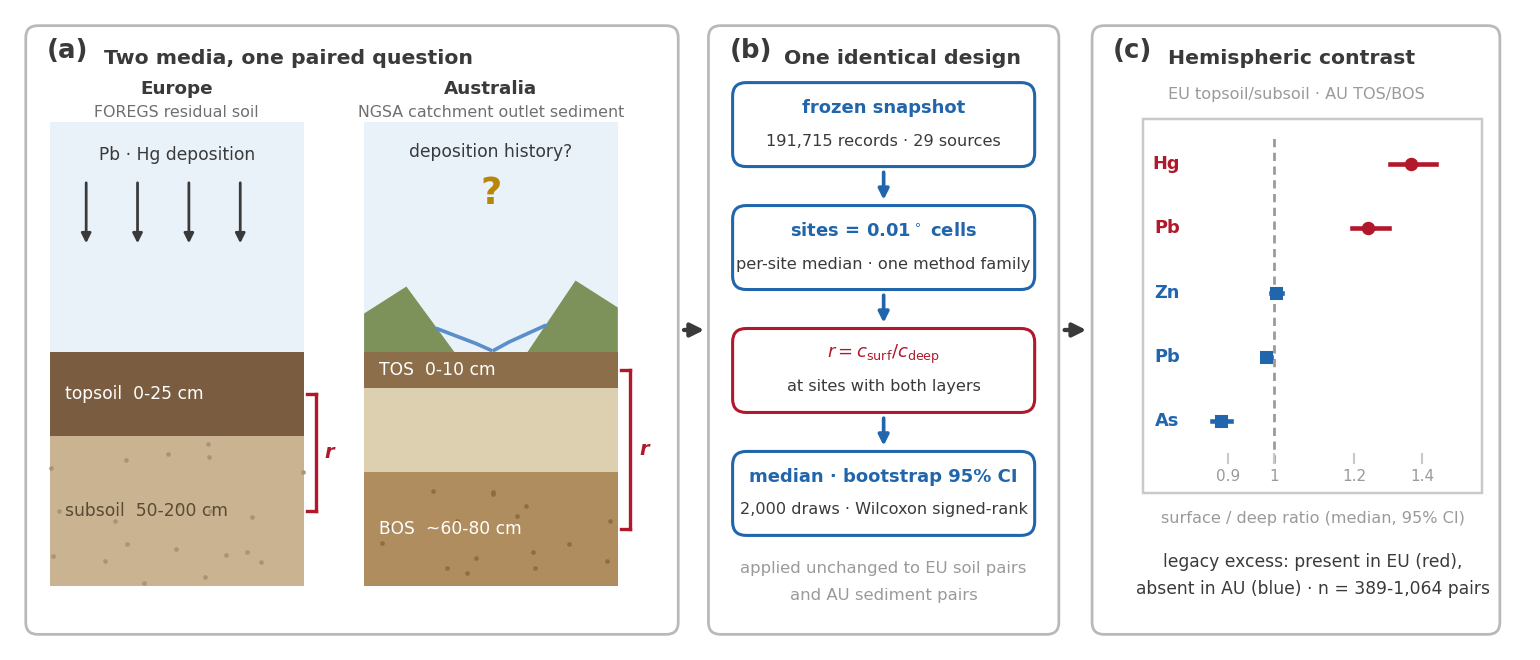
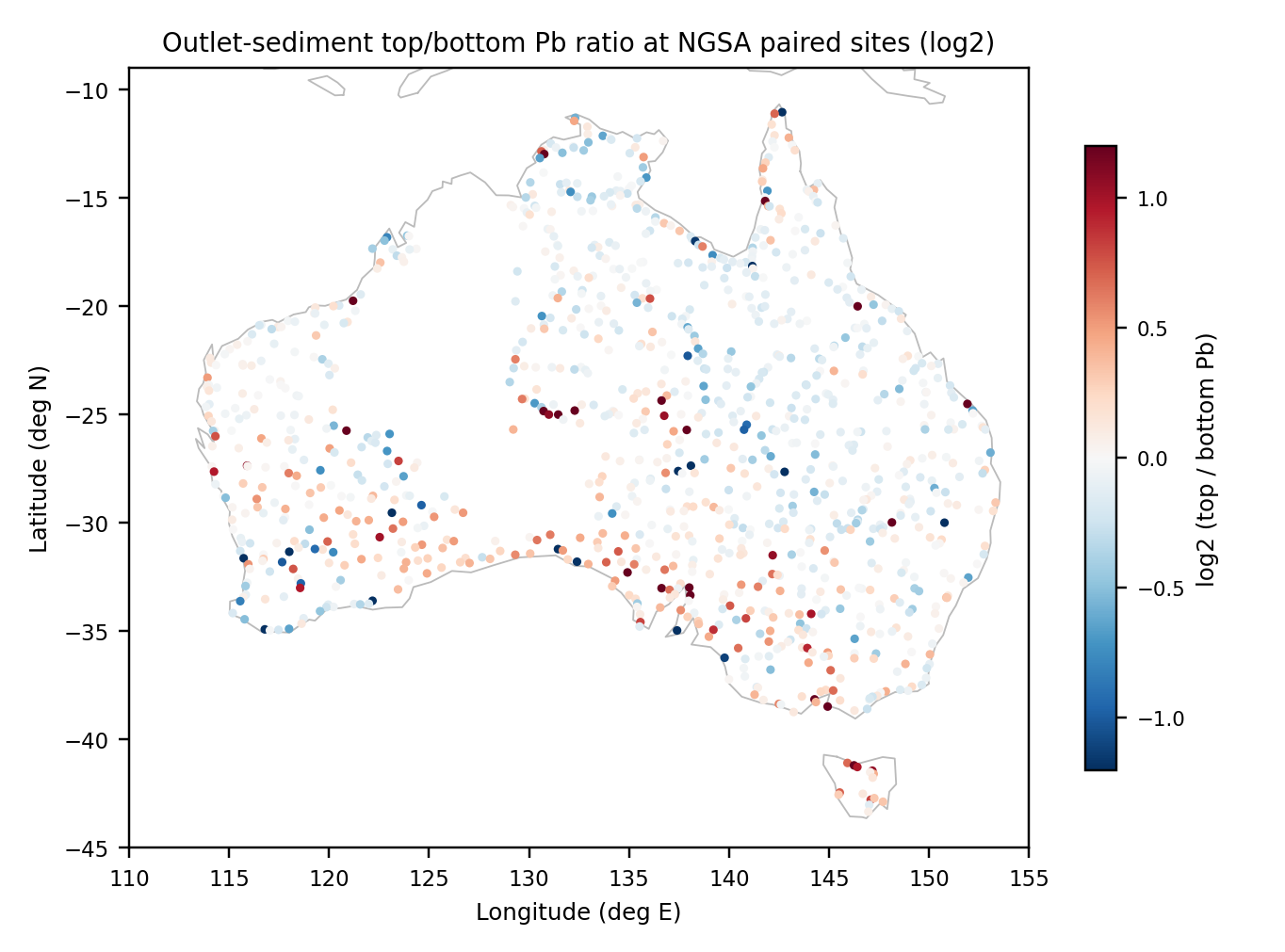
Finding: applying P1’s paired design unchanged to 1,064 NGSA sites in Australia gives a Pb top/bottom ratio of 0.982 — no European-style enrichment — while As shows surface depletion (0.886). The reference element Zn sits at ≈1 on both continents, so the contrast is not an artefact of the paired design. The result supports treating surface enrichment of legacy metals as a regional signature of Northern Hemisphere industry, and supplies the Southern Hemisphere baseline needed to evaluate the Minamata Convention.

P2 methods figure
METHODSTwo media, one paired question: European soil profiles vs Australian catchment sediments, same design
P2 results figure
RESULTMap of top/bottom Pb ratios at paired NGSA sites: Australia close to white = no enrichment, the counterpart to P1’s red Europe
P3
Same soil sample, two methods, up to threefold apart: quantifying and converting cross-method offsets QUESTIONHow far apart can total content by XRF and extractable content by acid-digestion ICP-MS be on the same sample? Can a validated transfer model merge the two kinds of data?
9 pages · 5 figures, 3 tables ES&T / Geostandards GGR Read the PDF ↗

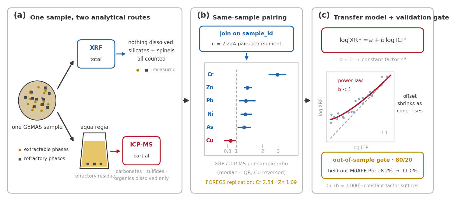
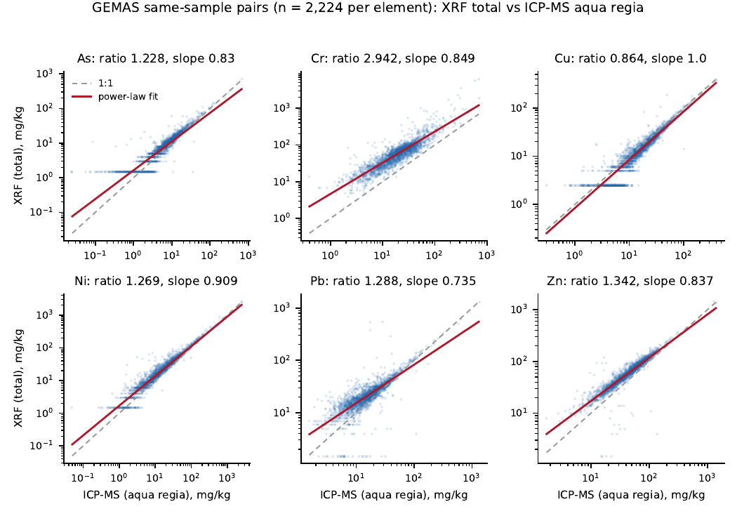
Finding: 2,224 same-sample duplicate measurements in GEMAS show that the method offset depends on element and concentration: Cr differs by 2.94×, while Cu shows a reverse offset (0.86). A log-log power-law transfer model validated on an 80/20 hold-out cuts the Pb prediction error from 18.2% to 11.0%; the independent FOREGS survey reproduces the same kind of offset (Cr 2.54). The paper proposes five minimum method-metadata standards — above all, record the analytical method completely, or cross-source conversion and merging cannot be done reliably.

P3 methods figure
METHODSOne sample, two analytical routes → same-sample pairing → transfer model and hold-out validation gate
P3 results figure
RESULTSix-element scatter of 2,224 same-sample pairs: red line = power-law fit, Cr sits almost 3× off the 1:1 line
P4
Do two independent surveys agree at the same location? Ground validation for the global arsenic map QUESTIONThe Science 2020 global groundwater-arsenic risk map explicitly lacks independent ground validation. How far apart are the arsenic readings of two mutually independent continental surveys in the same grid cell?
9 pages · 5 figures, 3 tables Environment International / Water Research Read the PDF ↗

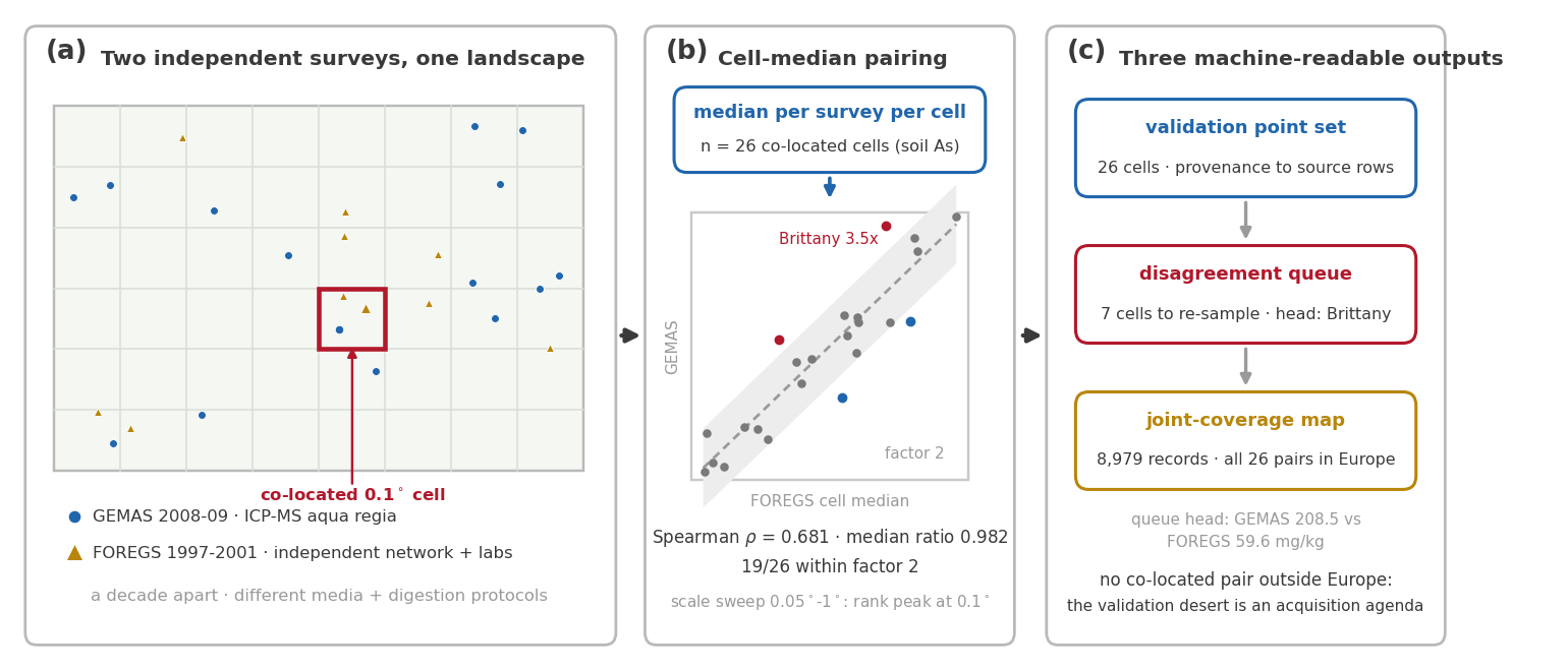
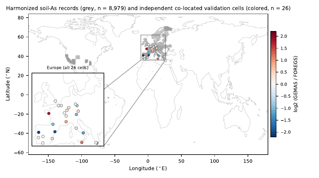
Finding: across the 26 co-located 0.1° cells shared by GEMAS and FOREGS the median ratio is 0.982 — the two surveys agree to within 2% at the same sites — and 73% of cells fall inside a factor-of-2 band. For the 7 discordant cells the pipeline automatically generated a re-sampling queue, led by Brittany with a 3.5× discrepancy; a scale scan shows 0.1° coincides with the peak of rank correlation, so the grid scale is data-driven. Such co-located validation is currently possible only in Europe — that “validation desert” is itself an explicit acquisition agenda.

P4 methods figure
METHODSTwo independent surveys → co-located cell pairing → three machine-readable products
P4 results figure
RESULTGlobal validation map: grey = 8,979 georeferenced As records, coloured dots = 26 co-located cells (all in Europe = the validation desert)
P5
Can zero tuning recover known oceanography? GEOTRACES profile extraction and method audit QUESTIONCan a generic statistical layer with no oceanographic assumptions automatically recover known ocean structure from 18,563 heterogeneous seawater records — and tell how heterogeneous the data can get before merging stops being appropriate?
9 pages · 5 figures, 1 table Marine Chemistry / ESSD Read the PDF ↗

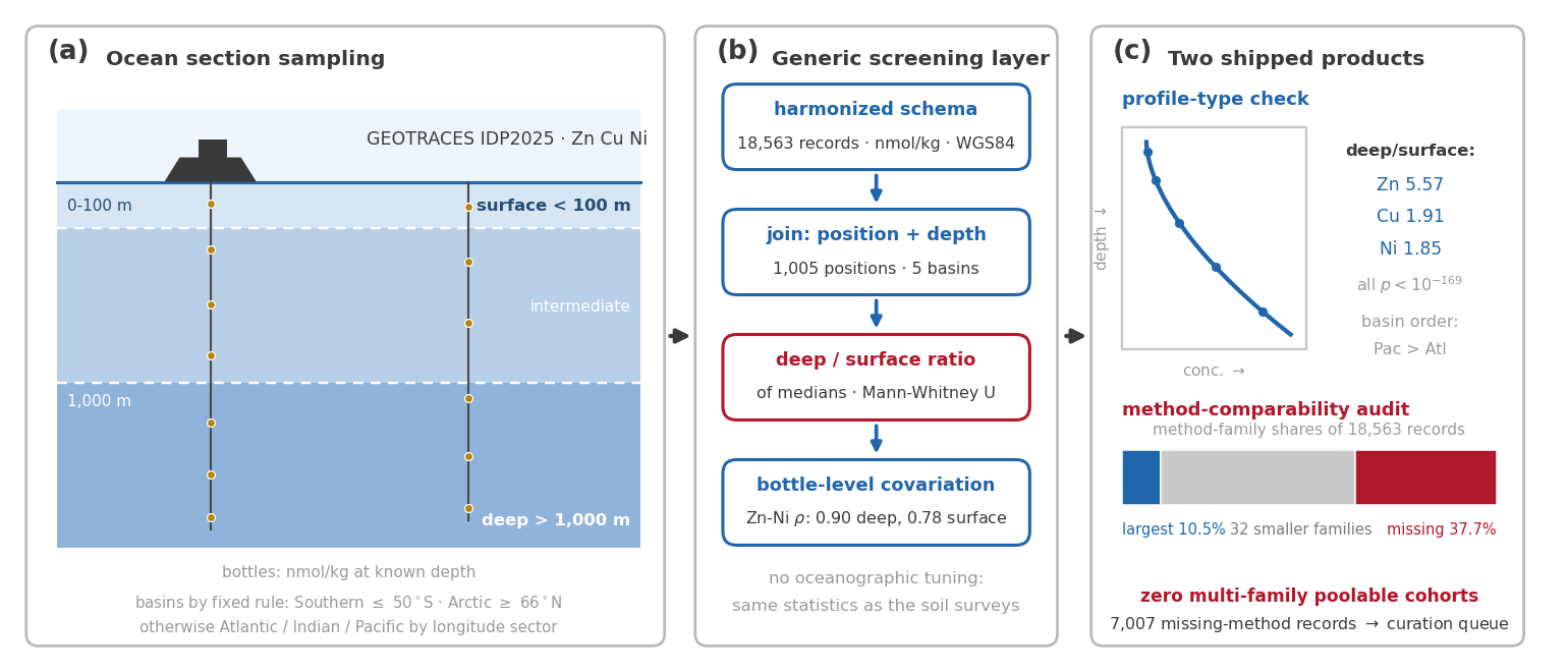
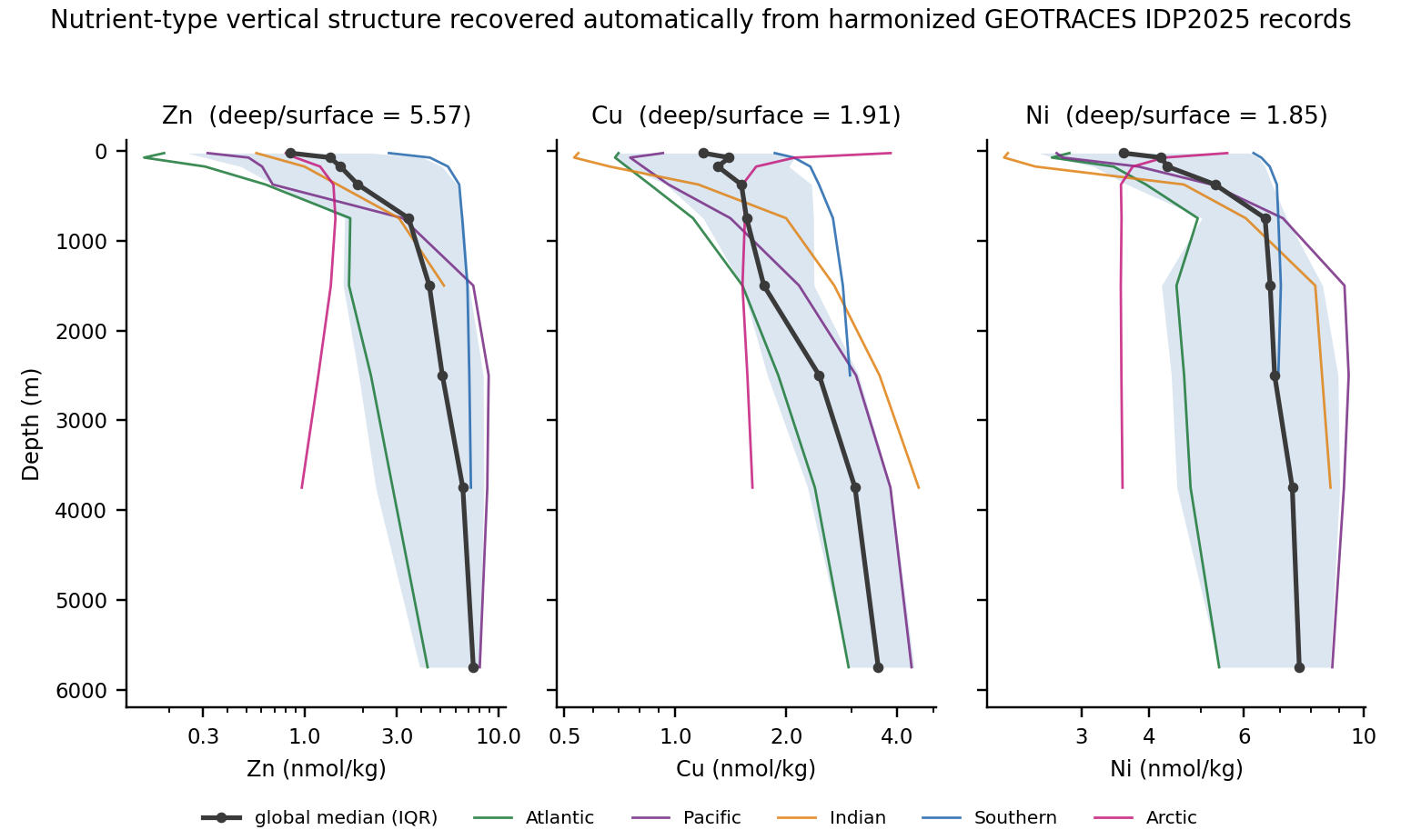
Finding: with no oceanographic prior and no tuning, nutrient-type profiles are recovered: Zn deep/surface 5.57×, basins ordered Pacific 24.5× > Atlantic 13×, consistent with water-mass age differences; the Arctic shows a river-influenced surface reversal; deep-water Zn–Ni correlation reaches ρ=0.90, consistent with remineralization coupling. The method audit shows that the best-covered of 33 resolvable method families accounts for only 10.5% of records, another 37.7% lack method metadata altogether, and the number of multi-source combinations that can be pooled directly is 0 — the corresponding gap list has been compiled into a repair queue for the data custodians.

P5 methods figure
METHODSOcean section sampling → generic screening layer (the same statistics as the soil papers) → two products
P5 results figure
RESULTZn/Cu/Ni depth profiles: black = global median, coloured lines = five ocean basins — the textbook structure emerges on its own

Compared with existing databases, where is the advantage?

Existing databases are positioned differently (all figures below verified on their official pages, accessed 2026-08-20): the large compilations win on coverage but mostly keep the format of the original publication; the thematic databases are well standardized but usually limited to one medium or one continent. GGA does not compete on volume — its point is the unified data layer that is missing between these resources.

GEOROC / DIGISLITERATURE COMPILATION · ROCK

The global igneous/metamorphic rock literature compilation maintained by the DIGIS programme of the Göttingen Academy: 42.7 million values / 707k samples / 23,520 publications. Strong in volume and literature coverage; numbers are compiled as published, with no cross-source unification of units or methods.

georoc.eu ↗
EarthChem · PetDB · SESARDATA FEDERATION · SOLID EARTH

The NSF-funded solid-earth data federation operated by Columbia University’s LDEO: about 50 million values / >1 million samples; SESAR issues globally unique IGSN identifiers to >5 million physical samples. Strong in sample registration and long-term archiving; each member database keeps its original published accounting.

earthchem.org ↗
USGS NGDBNATIONAL ARCHIVE · USA

The U.S. Geological Survey’s national geochemical archive since 1962: 1.524 million samples / >59 million determinations. Strong in sampling density and time span within the United States; 108 analytical methods and 25 laboratories coexist, with method names recorded but no unified comparable layer.

mrdata.usgs.gov ↗
GEOTRACES IDP2025SCIENCE PROGRAMME · SEAWATER ONLY

The intermediate data product of the international marine trace-element and isotope programme: 123 cruises / 4,097 stations / 2.2 million values, value-level quality flags, cross-over calibration between cruises. The benchmark for “unification done well” — but seawater only, with method information at cruise level.

geotraces.org/idp2025 ↗
Continental surveys ×6ONE CONTINENT · ONE CAMPAIGN

GEMAS (4,329 European agricultural and grazing-land soils), FOREGS (about 900 multi-medium stations across Europe), NGSA (1,315 Australian sediment stations), LUCAS (about 19k EU topsoil points), AfSIS (18,257 African samples), CGB (6,617 Chinese samples). Each is highly consistent internally (one method system + survey-level QC), but each covers one continent in one campaign, and they are not directly comparable with one another.

GEMAS ↗ · FOREGS ↗ · NGSA ↗ · LUCAS ↗ · AfSIS ↗
GGA (this project)UNIFIED LAYER · FOUR MEDIA · BOTH HEMISPHERES

Focused on cross-database unification rather than competing with anyone on size: 191,715 records from 29 sources and four media (soil / sediment / freshwater / seawater) organized into one auditable table of 129 fields, every record carrying a four-component confidence score; all five papers above were written directly from this table. It addresses exactly the gap named by the OneGeochemistry initiative — data fragmented across thousands of databases and almost impossible to reuse.

Full comparison with all sources ↗
CapabilityLarge compilations
EarthChem · GEOROC · NGDB
Thematic surveys
GEMAS · FOREGS · GEOTRACES …
GGA (this project)
Unified units and coordinates out of the boxcompiled as publishedunified within a survey, differs between surveysmg/kg + WGS84 across the whole database
One table across mediaseparate databases per mediummostly one medium / one continentsoil · sediment · water · rock in one table
Method metadata and cross-method conversionmethod names onlyconsistent within one method systemmethod-family labels + hold-out-validated transfer models
Record-level provenanceto publication / dataset levelto survey level100% row-level SHA-256 hash chain
Record-level license labelsdataset or page leveldataset level100% coverage, filter rows for redistribution
Record-level confidence scorevalue-level QC flags (e.g. GEOTRACES)four-component score travels with every record into analysis
Gaps delivered as a productmachine-readable acquisition priority queue

✓ provided · ◐ partly · — not provided. This is a positioning table, not a ranking: compilations excel at volume and archiving, surveys at internal consistency; GGA supplies the unified layer missing between them. The comparison uses the frozen paper snapshot (191,715 records / 29 sources); the latest 2026-08-19 production run has reached 199,730 records / 35 sources — the two tallies are kept separate and never mixed. Sources for every item are in the capability matrix below and in database-comparison.md.

What is the unified layer good for? Six questions researchers actually run into, compared one by one:

Q1 Can the data be analysed as soon as it is downloaded?Do units, coordinates and field formats still need cleaning source by source?
Compilation databases usually keep the published format; units, detection-limit definitions and coordinate datums differ between sources, and analysis is typically preceded by weeks of per-source cleaning (OneGeochemistry’s summary: “almost impossible to reuse”)
Every record already unified to mg/kg + WGS84 in one 129-field table, four media queried together; new media and sources join under the same field specification. P2 reused the same script and finished a second continent the same day
Q2 Can results from different methods be merged directly?XRF measures total content, acid-digestion ICP measures a partial extraction — mixing them blindly introduces systematic bias
NGDB holds 108 methods but mostly keeps only their names; literature compilations often lack method information altogether — mixing the same element can be off by 3×, and the database itself gives no warning
Every record is labelled with its method family; the 36.3% lacking method information keep a per-record missing_reason; P3 adds hold-out-validated transfer models (measured Cr offset 2.94×)
Q3 Are the numbers trustworthy and traceable?When a value looks suspicious, can you go back to the original source record by record?
Usually traceable only to publication or dataset level: whether a single record changed between download and ingestion — and what changed — cannot be judged by an outside user
Row-level SHA-256 hash chain with 100% coverage; any number replays back to the original download; deterministic scripts replay the processing byte for byte; censored values are never guessed — 1,537 are kept explicitly
Q4 Can it be reused and republished legally?When merging sources into a derived product, is the license boundary of every record clear?
Licenses are usually stated at dataset or even page level: once several sources are mixed, the redistribution boundary of a derived product is often impossible to determine
Record-level license field with 100% coverage: filter rows to a redistributable subset that satisfies any required license combination
Q5 Where are the gaps, and what should be measured next?Can gap information support sampling plans directly?
Gaps are usually not a product — users typically discover missing data only when their analysis runs into a blank region
Gaps are compiled into a machine-readable acquisition priority queue (geojson): the Hg gaps of P2 and the “validation desert” of P4 both became the next round of sampling points
Q6 Is the reliability of each record visible?Does the quality judgement travel with the record into analysis, or stay in the database documentation?
Quality information mostly appears as dataset documentation, method codes or single quality flags, rarely as a composite score that accompanies individual records into analysis
Every record carries a four-component confidence score with 100% coverage, usable directly for filtering, sensitivity analysis and result audits

Full capability matrix (every figure with an official source):

SystemScaleMediaUnified units · schemaRecord-level licenseProvenance hashMethod metadataConfidence · QCCross-validationGap queue
GGA (this project)191,715 records / 29 sources / 7 metalsFour media in one 129-field schema (soil 80,709 · sediment 79,630 · water 31,376)✓ mg/kg + WGS84 + per-record lineage100%100% row-level SHA-256✓ method families + 36.3% missing, accounted per record✓ four-component confidence 100%; 1,537 censored values kept explicitly26 co-located cells (P4)✓ acquisition-priority geojson queue
GEOROC / DIGIS42.7M values / 707k samples / 23,520 publications1igneous · metamorphic rocks · minerals— (compiled as published)dataset level— (publication level)✓ analysis level
EarthChem · PetDB · SESAR≈50M values / >1M samples; SESAR >5M registered samples2solid earth (federation of six)— (original published accounting kept)dataset levelIGSN, sample level✓ analysis level
USGS NGDB1.524M samples / >59M determinations3rock / sediment / soil / ore (USA)— (108 methods, 25 labs coexist)public domain (dataset level)method names, no unified layer
GEOTRACES IDP2025123 cruises / 4,097 stations / 2.2M values4seawater onlyunified within product + cross-overdata-product level— (cruise level)✓ method linksvalue-level flags + 1σcross-over calibration (within product)
GEMAS (Europe)2,211 agricultural + 2,118 grazing-land samples / 33 countries5soil only (one campaign)unified within surveydataset levelsingle method systemsurvey-level QC
FOREGS (Europe)about 900 stations / 26 countries / 5 media (water · sediment · soil)5multi-medium (one continent, one campaign)unified within surveydataset levelsingle method systemsurvey-level QC
NGSA (Australia)1,315 stations / 2 depths / 81% of the continent5catchment sediment (one campaign)unified within surveyCC BY (dataset level)single method systemsurvey-level QC
LUCAS · AfSIS · CGBLUCAS 18,984–21,859 points; AfSIS 18,257 samples; China baseline network 6,617 samples5soil only (one campaign per domain)unified within surveydataset levelsingle method systemsurvey-level QC

Footnotes 1–5 and the source of every figure (URL + access date 2026-08-20 + original wording) are in research/database-comparison.md; the GGA row comes from column-level statistics of the frozen snapshot retest-acquisition-coverage-v12-6c221cf.

Scientific boundary: all five papers are screening-level: enrichment ≠ a pollution verdict, profile shape ≠ proof of mechanism. All five passed the seven-item a–g quality audit (data plausibility / narrative consistency / typesetting / data completeness / terminology / figure standards / table standards), and still require expert human review before formal submission; every number can be replayed deterministically from the frozen snapshot with seeded scripts. Full roadmap: five-paper-roadmap.md; comparison sources: database-comparison.md.

Watch · 3 Minutes

3-minute demo: the approach and mechanisms first, then a real run

Chinese narration with Chinese subtitles. 00:00–01:22 walks through the research question, the mechanism overview, the loop state machine, the adversarial audit and a live agent run using the final-round slides; 01:22–02:52 is a real run — hands-on use of the World / China / Europe / United States atlases, and the 1986–2024 temporal evolution atlas playing automatically.

Downloads

Materials

One main slide deck (the HTML version used at the final, plus a PDF), one poster, one video, two written introductions and one technical appendix. The presentation materials are in Chinese; the code, README and papers are in English.